Epitol

Malcolm H. Lader, OBE, LLB, DSc, MD, PhD, FRCPsych, FMedSci

• Emeritus Professor of Clinical Psychopharmacology,
• King? College London, Institute of Psychiatry,
• London, UK

In a fixed level test medicine man dr dre buy generic epitol 100mg on line, we either reject the null hypothesis or we fail to reject the null hypothesis treatment bulging disc buy epitol 100mg cheap. It is more or less true that we can fix all but one of the interrelated pa- rameters and solve for the missing one symptoms uterine cancer 100mg epitol amex. This treatment breast cancer purchase epitol 100mg, of course medicine lake mn buy genuine epitol on line, is called i sample size that a sample size analysis medicine show buy discount epitol 100mg online, because we have specified a required power and now gives desired find a sample size that achieves that power. The use of power or sample size analysis begins by deciding on interest- ing values of the treatment effects and likely ranges for the error variance. Use prior Interesting values of treatment effects could be anticipated effects, or they knowledge of could be effects that are of a size to be scientifically significant; in either system case, we want to be able to detect interesting effects. For each combina- tion of treatment effects, error variance, sample sizes, and Type I error rate, we may compute the power of the experiment. Sample size computation amounts to repeating this exercise again and again until we find the smallest sample sizes that give us at least as much power as required. Thus what we do is set up a set of circumstances that we would like to detect with a given probability, and then design for those circumstances. First, 95% confidence intervals for pairwise differences (on the log scale) should be no wider than. We must specify the means and error variance to compute power, so we use those from the preliminary data. One sample size criterion is to choose the sample sizes so that confidence intervals of interest are no wider than a max- imum allowable width W. W 2 this is an approximation because n must be a whole number and the quantity on the right can have a fractional part; what we want is the smallest n such that the left-hand side is at least as big as the right-hand side. We can compute a reasonable lower bound for n by substituting the upper E /2 percent point of a normal for t2. With a sample size of 10, there are 27 degrees of freedom for error, so we now use t. This is because changing the sample size affects df and also changes the degrees of freedom and thus the percent point of t that we t-percent point use. When the null hypothesis is true, the F-statistic follows an F-distribution with degrees of freedom from the two mean squares. When the null hypothesis is false, the F-statistic noncentral follows a noncentral F-distribution. Power, the probability of rejecting the F-distribution null when the null is false, is the probability that the F-statistic (which fol- when null is false lows a noncentral F-distribution when the alternative is true) exceeds a cutoff based on the usual (central) F distribution. The vertical line is at the 5% cutoff point; 5% of the Power computed area under the null curve is to the right, and 95% is to the left. We would reject the null at the 5% level if our F-statistic is greater than the cutoff. The noncentral F-distribution has numerator and denominator degrees of freedom the same as the ordinary (central) F, and it also has a noncentrality Noncentrality parameter ζ defined by P 2 parameter niα i i measures ζ =. The ordinary central i i• i F-distribution has ζ = 0, and the bigger the value of ζ, the more likely we are to reject H0. Thus there is a different al- ternative distribution for each value of the noncentrality parameter, and we will only be able to tabulate power for a selection of parameters. The first is to use Power curves power tables—figures really—such as Appendix Table D. There is a separate figure for each numerator degrees of freedom, with power on the vertical axis and noncentrality param- 7. Within a figure, each curve shows the power for a particular denominator degrees of freedom (8, 9, 10, 12, 15, 20, 30, 60) and Type I error rate (5% or 1%). To compute power, you first get the correct figure (according to numer- ator degrees of freedom); then find the correct horizontal position on the figure (according to the noncentrality parameter, shifted right for. Computing minimum sample sizes for a required sample sizes power is a trial-and-error procedure. We investigate a collection of sample iteratively sizes until we find the smallest sample size that yields our required power. On the log scale, the group means in the prelimi- 156 Power and Sample Size nary data were 2. Again trying to be conservative, recompute the sample size assuming that the error variance is. Power curves are Often there is not a curve for the denominator degrees of freedom that we difficult to use need, and even when there is, reading power off the curves is not very accu- rate. These power curves are usable, but tedious and somewhat crude, and certain to lead to eyestrain and frustration. A better way to compute power or sample size is to use computer soft- ware designed for that task. As of summer 1999, they also maintain a Web pagelisting power analysis capabilities and sources for extensions for several dozen packages. The user interfaces for power soft- ware computations differ dramatically; for example, in Minitab one enters the means, and in MacAnova one enters the noncentrality parameter. If we design for this alternative, then we will have at least as much power for any other alternative with two treatments D units apart. In some situations, we may be particularly interested in one or two contrasts, and less interested in other contrasts. In that case, we might wish to design our experiment so that the contrasts of particular interest had adequate power. The F-test has 1 and parameter for a N − g degrees of freedom and noncentrality parameter contrast P g 2 (i=1 wiαi) Pg 2. The basic problems are those of dividing fixed resources (there is never enough money, time, material, etc. Consider first the situation where there is a fixed amount of experimental material that can be divided into experimental units. Larger units have Subdividing the advantage that their responses tend to have smaller variance, since these spatial units responses are computed from more material. Smaller units have the opposite properties; there are more of them, but they have higher variance. There is usually some positive spatial association between neighboring areas of experimental material. Because of that, the variance of the average of k adjacent spatial units is greater than the variance of the average of k More little units randomly chosen units. For example, there may be an expensive or time-consuming analytical measurement that must be made on each unit. An upper bound on time or cost thus limits the number of units that can be considered. When units are treated and analyzed in situ rather then being physically separated, it is common to exclude from analysis the edge of each unit. This is done because treatments may spill over and have effects on neighboring units; ex- cluding the edge reduces this spillover. The limit arises because as the units become smaller and smaller, more and more of the unit becomes edge, and we eventually we have little analyzable center left. A second situation occurs when we have experimental units and mea- surement units. Are we better off taking more measurements on fewer units More units or or fewer measurement on more units? In general, we have more power and measurement shorter confidence intervals if we take fewer measurements on more units. For example, consider an experiment where we wish to study the possi- ble effects of heated animal pens on winter weight gain. We have g treat- Costs may vary ments with n pens per treatment (N = gn total pens) and r animals per pen. Let σ2 be the variation from pen to pen, and let 1 σ2 be the variation from animal to animal. However, there are some situations where un- equal sample sizes could increase the power for alternatives of interest. Suppose that one of the g treatments is a control treatment, say treatment 1, and we are only interested in determining whether the other treatments Comparison with differ from treatment 1. That is, we wish to compare treatment 2 to control, control treatment 3 to control. For such an experiment, the control plays a special role (it appears in all contrasts), so it makes sense that we should estimate the control response more precisely by putting more units on the control. In fact, we can show that we should choose group sizes so that the noncontrol treatments sizes (√ nt) are equal and the control treatment size (nc) is about nc = nt g − 1. A second special case occurs when the g treatments correspond to nu- merical levels or doses. For example, the treatments could correspond to four Allocation for different temperatures of a reaction vessel, and we can view the differences polynomial in responses at the four treatments as linear, quadratic, and cubic temperature contrasts effects. If one of these effects is of particular interest, we can allocate units to treatments in such a way to make the standard error for that selected effect small. Suppose that we believe that the temperature effect, if it is nonzero, is essentially linear with only small nonlinearities. Thus we would be most interested in estimating the linear effect and less interested in estimating the quadratic and cubic effects. In such a situation, we could put more units at the lowest and highest temperatures, thereby decreasing the variance for the linear effect contrast. If our assumptions about shape of the response and importance of different contrasts are incorrect, we could wind up with an experiment that is much less informative than the equal 7. For example, suppose we are near the peak of a quadratic Sample sizes response instead of on an essentially linear response. Then the linear contrast based on (on which we spent all our units to lower its variance) is estimating zero, and incorrect the quadratic contrast, which in this case is the one with all the interesting assumptions can information, has a high variance. Mathematically, the ratio of two independent chi-squares, each divided by their degrees of freedom, has an F-distribution; thus the F-ratio has an F-distribution when the null is true. When the null hypothesis is false, the error sum of squares still has its chi-square distribution, but the treatment sum of squares has a noncentral chi-square distribution. If Z1, Z2, · · ·, Zn are independent normal random variables with mean 0 and variance 1, then Z2 + Z2 + · · · + Z2 (a sum of squares) has a chi-square 1 2 n distribution with n degrees of freedom, denoted by χ2. Then i i the sum of squares Z2 + Z2 + · · · + Z2 has a distribution which is σ2 times a 1 2 n noncentral chi-square distribution with n degrees of freedom and noncentral- Pn 2 2 2 ity parameter i=1 δi /σ. Let χn(ζ) denote a noncentral chi-square with n degrees of freedom and noncentrality parameter ζ. In Analysis of Variance, the treatment sum of squares has a distribution that is σ2 times a noncentral chi-square distribution with g − 1 degrees of Pg 2 2 freedom and noncentrality parameter i=1 niαi /σ. When the null is false, the F-ratio is a noncentral chi-square divided by a central chi-square (each divided by its degrees of freedom); this is a noncentral F-distribution, with the noncentrality of the F coming from the noncentrality of the numerator chi-square. We will have six experimental units per fertilizer and will do our test at the 5% level. One of the fertilizers is the standard and the other two are new; the standard fer- tilizer has an average yield of 10, and we would like to be able to detect the situation when the new fertilizers have average yield 11 each. The probability of rejecting the null hypothesis when the null hypoth- esis is false is. The probability of failing to reject the null hypothesis when the null hypothesis is true is. The six types of tape were 1) brand A high cost, 2) brand A low cost, 3) brand B high cost, 4) brand B low cost, 5) brand C high cost, 6) brand D high cost. Each tape will be recorded with a series of standard test patterns, replayed 10 times, and then replayed an eleventh time into a device that measures the distortion on the tape. The distortion measure is the response, and the tapes will be recorded and replayed in random order. We have historical data on six subjects, each of whose estradiol concentration was measured at the same stage of the menstrual cycle over two consecutive cycles. In our experiment, we will have a pretreat- ment measurement, followed by a treatment, followed by a posttreatment measurement. Our response is the difference (post − pre), so the variance of our response should be about. Half the women will receive the soy treatment, and the other half will receive a control treatment. Nondigestible carbohydrates can be used in diet foods, but they may have Problem 7. We want to test to see if inulin, fructooligosaccharide, and lactulose are equivalent in their hydrogen production. Preliminary data suggest that the treatment means could be about 45, 32, and 60 respectively, with the error variance conservatively estimated at 35. Suppose that the true expected value for the contrast with coefficients (1,-2,1) is 1 (representing a slight amount of curvature) and that the error variance is 60. Factorial treatment structure ex- Factorials ists when the g treatments are the combinations of the levels of two or more combine the factors. We call these combination treatments factor-level combinations or levels of two or factorial combinations to emphasize that each treatment is a combination of more factors to one level of each of the factors. We have not changed the randomization; we create treatments still have a completely randomized design. It is just that now we are con- sidering treatments that have a factorial structure. We will learn that there are compelling reasons for preferring a factorial experiment to a sequence of experiments investigating the factors separately. Lynch and Strain (1990) performed an experiment with six treatments studying how milk-based diets and copper supplements affect trace element levels in rat livers. The six treatments were the combinations of three milk-based diets (skim milk protein, whey, or casein) and two copper supplements (low and high levels). Whey itself was not a treatment, and low copper was not a treatment, but a low copper/whey diet was a treatment. Nelson, Kriby, and Johnson (1990) studied the effects of six dietary supplements on the occur- rence of leg abnormalities in young chickens.

A classic picture of obstruction would appear urodynamically as an elevated intravesical pressure relative to a low urinary flow rate treatment using drugs purchase epitol 100mg otc. As a management option treatment neuroleptic malignant syndrome generic 100 mg epitol with visa, surgery is typically performed in the operating room setting medicine 6 year course purchase genuine epitol on-line, requires anesthesia and is associated with the greatest risks for morbidity and higher costs treatment dvt purchase 100 mg epitol otc. The clinical data supporting the use of these surgical procedures including several comparative trials are herein reviewed 4d medications order genuine epitol line. Systematically acute treatment cheap epitol 100 mg amex, current evidence describing the background literature and outcomes for each procedure have been considered. For reference, detailed evidence tables reviewing the studies evaluated by the Panel are provided in Appendix A8. Single-group Cohort Studies the 12 single-group cohort studies examining open prostatectomy that were identified in this review generally included subjects with larger glands or patients needing surgery for bladder or other pelvic or inguinal conditions. Approximately half of the studies were retrospective series and a number of the studies examined only intra- and peri-operative outcomes and complications without examination of efficacy and effectiveness outcomes. Follow-up intervals ranged from the immediate postoperative period up to 191 192-197 198 11 years. The various techniques of open prostatectomy included transvesical and retropubic. Bernie 200 et al compared the three techniques, namely transversica, retropubic, and perineal. Postvoid residual and Qmax also improved significantly in all studies examining this outcome at mean follow-up up to three years. In the only study of sexual 194 function after surgery, a significant increase in sexual desire and overall satisfaction was observed. Perioperative and Short-Term Outcomes Intraoperative blood loss more than 1000 mL was reported in several studies using the 191, 200, 202 retropubic approach. Hospital stay for open prostatectomy ranged between five to seven 191, 193, 195-197, 199, 200 days in many studies; however, the mean length of stay was approximately 11 days in 192, 202 other studies of transvesical prostatectomy. Bernie and Schmidt compared hospital stays among surgical approaches and reported five and six days for retropubic and suprapubic approaches, 200 respectively. Longer-term Complications Mortality was infrequently reported in these studies and perioperative death rates were low 193, 195, 202 (≤1%) and generally related to cardiovascular disease. In the large (n=1,800) series by Serretta 199 and colleagues, one perioperative death was reported. The discovery of incidental prostate cancer in 193 201 192 195 202 resected specimens was reported at rates of 2%, 3. Bladder neck contracture was reported at 3% to 6% and in 200 one of six subjects undergoing perineal open prostatectomy in a single series. Laparoscopic Prostatectomy Cohort Studies with a Comparison Group A single cohort study (n=60) compared consecutive patients undergoing laparoscopic 203 prostatectomy with a consecutive retrospective cohort of open prostatectomy. Sotelo reported a mean operative time of 156 minutes (range 85 to 380) and a mean 198 blood loss of 516 mL (range 100 to 2500 mL). Large prostate 213, 215 211 214 glands were examined in several studies: >100 g, 40 to 200 g and 70 to 220 g. The percentage of subjects in urinary retention at baseline was generally not reported; in two studies such subjects were 210, 211 excluded from study participation. Few details were provided on participant © Copyright 2010 American Urological Association Education and Research, Inc. Follow-up was generally less than one year, 217, 218, 220, 227 although several included longer follow-up. A significant percentage of subjects were in urinary retention at baseline in several studies, although this information was infrequently 217, 221, 222, 224 reported at baseline. Follow-up interval ranged from six weeks to three years, with only two studies 246, 249 providing data for longer than 12 months. Mean age of study participants ranged between 64 and 237, 243, 251 79 years, and the mean age was 75 years or greater in several studies. Men in urinary retention were excluded in some studies, while in others a 237, 243, 244, 251 significant pecentage had chronic urinary retention. Efficacy and Effectiveness Outcomes Similar to the analysis of the surgical therapies in the 2003 analysis, the symptom score and peak-flow data were available for most laser treatments and QoL scores were available for most treatments. Monoski and colleagues (2006) examined the relationship between preoperative urodynamic parameters and 266 outcomes in 40 patients in urinary retention. Postoperatively, subjects with detrusor overactivity had more voiding symptoms than those without detrusor overactivity. Men without impaired detrusor © Copyright 2010 American Urological Association Education and Research, Inc. While there are no direct comparisons between the various laser technologies, the improvements in symptom scores appear to be comparable to other surgical therapies and durable to five years. Data from a single investigator suggest that the QoL assessment in the interval between one year and six years follow-up is still improved but variable, as reported scores ranged between -2. Single group cohort studies using holmium ablation of the prostate report that the improvements in QoL scores noted at 258 three months postoperatively were sustained at seven years although no statistics were provided. In the single cohort study that included 54 patients improvement was found in the QoL score at one-year however, due to 253 limited data, conclusions about this modality cannot be drawn. Summary Although data are limited, the QoL score improved post-laser therapy when evaluated at one- and two-year follow-up regardless of the procedure type (except for thulium, for which conclusion could not be drawn). In general, 258, 259, 261 there were no significant differences between groups at one-year. When a holmium laser was used to ablate the prostate, a single-group cohort study reported that the improvements in QoL scores noted at three 272 months postoperatively were sustained at seven years although no statistics were provided. The outcomes associated with the thulium laser were reported for 54 253 patients in a single-cohort study and suggested a significant improvement in the Qmax at 12 months. All surgical therapies provided similar outcomes over time with regard to peak flow. A single-cohort study reported that the improvement in post-void residual was not related to the size of the prostate gland. The studies involving thulium laser therapy did not report the outcomes for the post-void urinary residuals. Changes following laser therapy may impact the outer diameter of the prostate as well as the inner lumen of the urethra. Thus total prostate volume measured after ablative therapies may not accurately reflect the amount of prostate tissue removed or the changes in the prostate. Studies concerning holmium lasers do not address changes in prostate volume following 258- therapy but do refer to weight of resected tissue. There is no information concerning the impact of the thulium laser on prostate volume or the impact of any laser therapy on the transition zone volume. The literature does not contain information concerning the impact of the various laser therapies on the detrusor pressures at maximum flow. Randomized controlled studies of the holmium laser compared to open prostatectomy found a total withdrawal rate of 38. The concerns for mortality rates associated with laser therapies are referred to the section addressing mortality for all surgical therapies. Intraoperative, immediate, postoperative, and short-term complications involve a broad spectrum of events and reporting rates may be based on subjective thresholds. The ability to directly compare laser therapies with respect to the operative time is constrained by the fact that each laser modality seems to select from patient populations with different baseline characteristics and seldom selects the same comparison therapy as a control. This is in contrast to a cohort comparison study that reported operative times were similar despite greater tissue resection with holmium enucleation. However, other studies reported enucleation times of 86 minutes in a large series, which was 255 improved from 112 minutes in their initial series of 118 cases. The longest mean operative time was reported in a series by Kuo et al (2003) (133. A single-cohort study reported that the average weight of prostate tissue resected 294 was 11 g and the procedure required an average operative time of 47 minutes. The sole study for the thulium laser is a single-cohort study reporting an operative time of 52 minutes in men with a mean pretreatment prostate volume of 32 mL. In a small single-cohort study of the outcomes associated with the thulium laser, no patient required © Copyright 2010 American Urological Association Education and Research, Inc. The published data in the interval from the 2003 analysis of the literature does not provide sufficient information to assess a change in risk. This rate is higher than expected from other transurethral technologies available today and the reason for the difference is not clear. Minimally invasive and surgical procedures induce irritative voiding symptoms immediately after and for some time subsequent to the procedure. Periprocedure and postprocedure adverse events associated with voiding symptoms include frequency, urgency, and urge incontinence and are categorized as postprocedure irritative adverse events. Such events are reported more often following heat-based therapies than following tissue-ablative surgical procedures. Because they impact QoL, irritative events are important and warrant documentation. Unfortunately, all patients will have some symptoms during the healing process immediately following the procedure. Because there is no standard for reporting this outcome, some studies reported these early symptoms while others did not. Further, because it is not possible to stratify these complaints according to severity, it is not possible to compare the degree of bother of these symptoms across therapies. Unfortunately, some studies report protocol-required or investigator option episodes of postprocedure catheterization while others report only catheterization performed for inability to urinate. Further, new technologies are resulting in earlier removal of catheters with much shorter hospital stays. The earlier attempts to remove the catheter are likely to increase the reported rates of repeat catheterization compared to historical rates associated with other technologies and longer hospital stays. Randomized controlled studies also showed a shorter length of 263, 294 stay for patients treated with holmium resection of the prostate. This wide range is believed to be a reflection of the change in technology over the review period as the laser energy increased in increments from 40W to 100W over time. In addition, various protocols in select institutions facilitated early discharge from the hospital. The average hospital stay reported in the study 253 utilizing the thulium laser was 3. The category urinary incontinence represents a heterogeneous group of adverse events, including total and partial urinary incontinence, temporary or persistent incontinence, and stress or urge incontinence. Secondary procedures, defined as interventions rendered by the treating physician for the same underlying condition as the first intervention, are challenging to classify. Examples of such procedures include initiation of medical therapy following a minimally invasive or surgical treatment, minimally invasive treatment following surgical intervention, or surgical intervention following a minimally invasive treatment. First, the threshold for initiating a secondary procedure varies by patient, physician, and the patient-physician interaction. In the absence of clearly defined thresholds for the success or failure of an initial intervention, secondary procedures are initiated on the basis of subjective perceptions on the part of either patients or treating physicians, which may not be reproducible or comparable between investigators, trials, or interventions. In many cases, patients involved in treatment trials feel a sense of responsibility toward the physician; given this commitment, patients may abstain from having a secondary procedure even through they may feel inadequately treated. Conversely, patients involved in treatment trials are more closely scrutinized in terms of their subjective and objective improvements; therefore, failures may be recognized more readily and patients may be referred more quickly for additional treatment. Moreover, the duration of trials and follow-up periods both affect rates at which secondary procedures are performed. Thus, although patients receiving long- term follow-up are at greater risk for treatment failure than those followed for short periods, it is virtually impossible to construct Kaplan-Meier curves or perform survival analyses for secondary procedure rates. As a result, the estimates for secondary procedure rates should be viewed with caution. Reoperation rates following various laser therapies are inconsistently reported, often due to the limited length of follow-up or the small numbers of patients in these studies. Inclusion and exclusion criteria were generally similar across studies, excluding subjects with prior pelvic surgery, prostate cancer, and neurologic disorders. The mean age of study participants was similar across studies, ranging between approximately 65 and 70 years. There was significant variation in Qmax at baseline, ranging from two to 20 mL per second in individual treatment groups. There was also much variation in preoperative prostate gland size: one study examined small glands (mean prostate volume of treatment 305 groups ranged from 24 to 34 mL), while another examined larger glands (mean of treatment groups, 308 54 mL and 63 mL). Qmax improved in both treatment groups; however the between-group error was inconsistent across studies. In studies where post-void residual was compared between treatments, no significant differences were found, with improvements noted with both 302, 304, 306, 308-311 treatments. Safety Outcomes Withdrawals and Treatment Failure Withdrawal rates were only reported in three of the 10 trials, with high rates of attrition when follow-up was two years or more. Mortality rates were low, largely due to cardiovascular disease, and never attributed to the surgical intervention. Longer-term Adverse Events Urethral stricture and bladder neck stenosis were uncommon and occurred with both treatments. Total sample size ranged between 40 and 240 subjects and follow-up intervals 319 323 varied between three weeks and 21 months. Cohort Studies with a Comparison Group 325, 326 We identified two cohort studies with comparison groups. Methods for recruiting subjects or identifying the study cohort were not generally reported. Sample size varied greatly (ranging from 21 to 1,014 327, 335, 336, 339, 342-344 participants), and seven studies had a sample size greater than 200 participants.

When we analyze these data medications qd generic 100 mg epitol free shipping, we can take the average or sum of the two patches on each branch as the response for the branch symptoms uterine fibroids cheap 100 mg epitol fast delivery. Experience and intuition lead the ex- perimenter to believe that branches on the same cycad will tend to be more alike than branches on different cycads—genetically symptoms 9dpiui buy generic epitol 100mg on-line, environmentally treatment improvement protocol buy epitol 100 mg online, and perhaps in other ways medications and breastfeeding purchase epitol paypal. The table makes it appear as though the first unit in every block received the water treatment medicine qhs best purchase epitol, the second unit the spores, and so on. The water treatment may have been applied to any of the three units in the block, chosen at random. You cannot determine the design used in an experiment just by looking at a table of results, you have to know the randomization. There may be many 318 Complete Block Designs Follow the different designs that could produce the same data, and you will not know randomization to the correct analysis for those data without knowing the design. The treatments could simply be g treatments, treatment or they could be the factor-level combinations of two or more factors. All of these treatment structures can be incorporated when we use blocking designs to achieve vari- ance reduction. This experiment was conducted to determine the requirements for protein and the amino acid threonine. Specifically, this experiment will examine the factorial combinations of the amount of protein in diet and the amount of threonine in diet. On the second day after arrival, all rats were weighed, and the rats were separated into five groups of 40 to provide groupings of approximately uniform weight. Body weight and food consumption were measured twice weekly, and the response we consider is average daily weight gain over 21 days. Initial body weight is a good predictor of body weight in 3 weeks, so the rats were blocked by initial weight in an attempt to find homogeneous groups of units. This decrease in error variance is achieved by finding groups of units that are homogeneous (blocks) and, in effect, Block when you repeating the experiment independently in the different blocks. We would like to group into blocks on the basis of homogeneity of the responses, but that is not possible. Instead, we must group into blocks on the basis of other similarities that we think may be associated with responses. For example, you need milk to make cheese, and you get a new milk supply every day. If your batches are such that you can make several types of cheese per batch, then blocking on batch of raw material is a natural. For example, some units may be located in one city, and other units in a second city. Or, some units may be in cages on the top shelf, and others in cages on the bottom shelf. It is common for Block spatially units close in space to have more similar responses, so spatial blocking is also common. That is, some units may be treated or measured at one time, and other units at another time. For example, you may only be able to make four measurements a day, and the instrument may need Block temporally to be recalibrated every day. As with spatial grouping, units close in time may tend to have similar responses, so temporal blocking is common. In general, any source of variation that you think may influence the history blocks response and which can be identified prior to the experiment is a candidate for blocking. To complete the model, we must decide which terms are random and which are fixed; we must also decide whether to use the standard additive model given above or to allow for the possibility that treatments and blocks All reasonable interact. Panels (a) and (b) assume the blocks analysis are fixed, and panels (c) and (d) assume the blocks are random. Panels (a) and (c) assume that blocks do not interact with treatments (as in the standard model above), and panels (b) and (d) include an interaction between blocks and treatments. In all four cases, we will use the (r − 1)(g − 1) degree of freedom term below treatments as the denominator for treatments. This is true whether we think that the treatments are fixed or random; what differs is how this denominator term is interpreted. In panel (d), this term is the block Denominator for by treatment interaction and is again the natural denominator for treatments. Instead, we must use the freedom interaction or block by treatment interaction as a surrogate for error and recognize that this error surrogate error may be too large if interaction is indeed present. Thus we will arrive at the same inferences regardless of our assumptions on randomness of blocks and interaction between treatments and blocks. The computation of estimated effects, sums of squares, contrasts, and so on is done exactly as for a two-way factorial. The reason for this goes back to thinking of F-tests as Do not test approximations to randomization tests. More pragmatically, we blocked because we believed that the units within blocks were more similar, so finding a block effect is not a major revelation. To some degree this assumption is forced on us, be- cause as we saw from the Hasse diagrams, there is little we can do besides assume additivity. When the treatments have a factorial structure, we could Standard model have a model with blocks random and interacting with the various factors. In has blocks such a model, the error for factor A would be the A by block interaction, the additive error for factor B would be the B by block interaction, and so on. However, the standard model allows treatment factors to interact, whereas blocks are still additive. When there is transformable nonadditivity, reexpressing the data on the appropriate scale can make the data more additive. When the data are more additive, the term that we use as error contains less interaction and is a better surrogate for error. As discussed above, the F-test for blocks does not correspond to freedom a valid randomization test for blocks. Even if it did, knowing simply that the blocks are not all the same does not tell us what we need to know: how much have we saved by using blocks? Units almost always translate to time or money, so reducing N by blocking is one good way to save money. Efficiency is denoted by E with a subscript to identify the designs be- ing compared. The first part is a degrees of freedom adjustment; variances must be estimated and we get better estimates with more degrees of freedom. The second part is the ratio of the error variances for the two different designs. The efficiency is determined primarily by this ratio of variances; the degrees of freedom adjustment is usually a smaller effect. Observe that even in this fairly small experiment, the loss from degrees of freedom was rather minor. Balance was helpful in factorials, and it is helpful in randomized Balance makes complete blocks for the same reason: it makes the calculations and inference inference easier easier. When the data are balanced, simple formulae can be used, exactly as for balanced factorials. When the data are balanced, adding 1 million to all the responses in a given block does not change any contrast between treatment means. If the treatments are themselves factorial, we can compute whatever type of sum of squares we feel is appro- Treatments priate, but we always adjust for blocks prior to treatments. The reason is that adjusted for we believed, before any experimentation, that blocks affected the response. This ordering for sums of squares and testing does not affect the final estimated effects for either treatments or blocks. There are experimental situations with more than one source of extraneous variation, and we need designs for these situations. One population control method is to addle eggs in nests to prevent them from hatching. This method may be harmful to the adult females, because the females fast while incubating and tend to incubate as long as they can if the eggs are unhatched. The birds in the study will be banded and observed in the future so that survival can be estimated for the two treatments. It is suspected that geese nesting together at a site may be similar due to both environmental and interbreeding effects. We would like each treatment to be used equally often at all sites (to block on populations), and we would like each treatment to be used equally often with young and old birds (to block on age). There are two blocking factors in a Latin Square, and these are represented by the rows and columns of the square. Thus in the goose egg example, we might have rows one once in each row and two be different nesting sites, with column one being young birds and and column column two being older birds. Using the two by two square above, treatment A is given to the site 1 old female and the site 2 young female, and treatment B is given to the site 1 young female and the site 2 old female. Second, Latin Squares generally have relatively few degrees of freedom for estimating error; this problem is particularly serious for small designs. Third, it may be difficult to obtain units that block nicely on both sources of variation. For example, we may have two sources of variation, but one source of variation may only have g − 1 units per block. We need to block on subjects, because each subject tends to respond differently, and we need to Crossover design block on time period, because there may consistent differences over time due has subject and to growth, aging, disease progression, or other factors. A crossover design time period blocks has each treatment given once to each subject, and has each treatment occur- ring an equal number of times in each time period. With g treatments given to g subjects over g time periods, the crossover design is a Latin Square. The concentration will typically start at zero, increase to some maxi- mum level as the drug gets into the bloodstream, and then decrease back to zero as the drug is metabolized or excreted. These time-concentration curves may differ if the drug is delivered in a different form, say a tablet versus a capsule. Bioequivalence studies seek to determine if different drug delivery systems have similar biological effects. We wish to compare three methods for delivering a drug: a solution, a tablet, and a capsule. There are three subjects, and each subject will be given the drug three times, once with each of the three methods. Because the body may adapt to the drug in some way, each drug will be used once in the first period, once in the second period, and once in the third period. Subject 1 2 3 1 A 1799 C 2075 B 1396 Period 2 C 1846 B 1156 A 868 3 B 2147 A 1777 C 2291 13. In principle, harder you assign treatments to units randomly, subject to the restrictions that each treatment occurs once in each row and once in each column, but effecting that randomization is harder than it sounds. This randomization starts with standard squares, which are squares with the Standard squares letters in the first row and first column in order. Then randomly permute all rows except the first, randomly permute all columns, and randomly assign Fisher-Yates the treatments to the letters. For g of 6, select a standard square at random, randomization randomly permute all rows and columns, and randomly assign the treatments to the letters. For g of 7 or greater, choose any square, randomly permute the rows and columns, and randomly assign treatments to the letters. Let yijk be the treatment, row, response from the unit given the ith treatment in the jth row block and kth and column column block. The standard model is effects 328 Complete Block Designs yijk = µ + αi + βj + γk + ǫijk, where αi is the effect of the ith treatment, βj is the effect of the j row block, and γk is the effect of the kth column block. The sum ••• i•• of squares for error is usually found by subtracting the sums of squares for treatments, rows, and columns from the total sum of squares. The Analysis of Variance table for a Latin Square design has sources for rows, columns, treatments, and error. We test the null hypothesis of no treatment effects via the F-ratio formed by mean square for treatments over mean square for error. Start with the total degrees of freedom g2 and Few degrees of subtract one for the constant and all the degrees of freedom in the model, freedom for error 3(g − 1). There is reasonable evidence against the null hypothesis that all three meth- ods have the same area under the curve, p-value. Note that this three by three Latin Square has only 2 degrees of freedom for error. We should ignore these, because period and subject are unrandomized blocking factors. Thus using multiple Latin Squares in a single estimates experiment is common practice. For example, we may believe that the period effects in a Some blocks can crossover design will be the same in all squares; this reuses the period blocks be reused across the squares. Replicated Latin Squares can reuse both row and column blocks, reuse neither row nor column blocks, or reuse one of the row or column blocks. Some blocks may Reusability represent small batches of material or time periods when weather is fairly depends on constant; these blocks may be unavailable or have been consumed prior to experiment and the second replication. Other blocks may represent equipment that could be logistics reused in principle, but we might want to use several pieces of equipment at once to conclude the experiment sooner rather than later. From an analysis point of view, the advantage of reusing a block fac- tor is that we will have more degrees of freedom for error. The risk when reusing a block factor is that the block effects will actually change, so that the assumption of constant block effects across the squares is invalid.

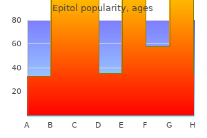
Best buy for epitol. Treating a Patient with Pneumonia? (TMC Practice Question) | Respiratory Therapy Zone.